Profiler
The profiler is a sampling profiler designed to analyze and visualize Noir programs. It assists developers to identify bottlenecks by mapping execution data back to the original source code.
Installation
The profiler is automatically installed with Nargo starting noirup v0.1.4.
Check if the profiler is already installed by running noir-profiler --version. If the profiler is not found, update noirup and install the profiler by reinstalling both noirup and Nargo.
Usage
Profiling ACIR opcodes
The profiler provides the ability to flamegraph a Noir program's ACIR opcodes footprint. This is useful for approximately identifying bottlenecks in constrained execution and proving of Noir programs.
"Approximately" as:
- Execution speeds depend on the constrained execution trace compiled from ACIR opcodes
- Proving speeds depend on the how the proving backend of choice interprets the ACIR opcodes
Create a demonstrative project
Let's start by creating a simple Noir program that aims to zero out an array past some dynamic index.
Run nargo new program to create a new project named program, then copy in the following as source code:
fn main(ptr: pub u32, mut array: [u32; 32]) -> pub [u32; 32] {
    for i in 0..32 {
        if i > ptr {
            array[i] = 0;
        }
    }
    array
}
Change into the project directory and compile the program using nargo compile. We are now ready to try out the profiler.
Flamegraphing
Let's take a granular look at our program's ACIR opcode footprint using the profiler, running:
noir-profiler opcodes --artifact-path ./target/program.json --output ./target/
The command generates a flamegraph in your target folder that maps the number of ACIR opcodes to their corresponding locations in your program's source code.
Opening the flamegraph in a web browser will provide a more interactive experience, allowing you to click into different regions of the graph and examine them.
Flamegraph of the demonstrative project generated with Nargo v1.0.0-beta.2:

The demonstrative project consists of 387 ACIR opcodes in total. From the flamegraph, we can see that the majority come from the write to array[i].
With insight into our program's bottleneck, let's optimize it.
Visualizing optimizations
We can improve our program's performance using unconstrained functions.
Let's replace expensive array writes with array gets with the new code below:
fn main(ptr: pub u32, array: [u32; 32]) -> pub [u32; 32] {
    // Safety: Sets all elements after `ptr` in `array` to zero.
    let zeroed_array = unsafe { zero_out_array(ptr, array) };
    for i in 0..32 {
        if i > ptr {
            assert_eq(zeroed_array[i], 0);
        } else {
            assert_eq(zeroed_array[i], array[i]);
        }
    }
    zeroed_array
}

unconstrained fn zero_out_array(ptr: u32, mut array: [u32; 32]) -> [u32; 32] {
    for i in 0..32 {
        if i > ptr {
            array[i] = 0;
        }
    }
    array
}
Instead of writing our array in a fully constrained context, we first write our array inside an unconstrained function. Then, we assert every value in the array returned from the unconstrained function in a constrained context.
This brings the ACIR opcodes count of our program down to a total of 284 opcodes:

Searching
The i > ptr region in the above image is highlighted purple as we were searching for it.
Click "Search" in the top right corner of the flamegraph to start a search (e.g. i > ptr).
Check "Matched" in the bottom right corner to learn the percentage out of total opcodes associated with the search (e.g. 43.3%).
If you try searching for memory::op before and after the optimization, you will find that the search will no longer have matches after the optimization.
This comes from the optimization removing the use of a dynamic array (i.e. an array with a dynamic index, that is its values rely on witness inputs). After the optimization, the program reads from two arrays with known constant indices, replacing the original memory operations with simple arithmetic operations.
Profiling proving backend gates
The profiler further provides the ability to flamegraph a Noir program's proving backend gates footprint. This is useful for fully identifying proving bottlenecks of Noir programs.
This feature depends on the proving backend you are using and whether it supports the profiler with a gate profiling API. We will use Barretenberg as an example here.
Flamegraphing
Let's take a granular look at our program's proving backend gates footprint using the profiler, running:
noir-profiler gates --artifact-path ./target/program.json --backend-path bb --output ./target -- --include_gates_per_opcode
The --backend-path flag takes in the path to your proving backend binary.
The above command assumes you have Barretenberg (bb) installed and that its path is saved in your PATH. If that is not the case, you can pass in the absolute path to your proving backend binary instead.
Flamegraph of the optimized demonstrative project generated with bb v0.76.4:
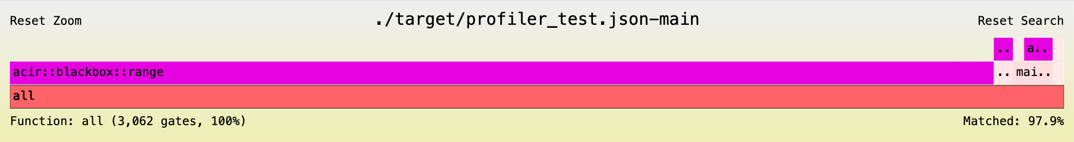
The demonstrative project consists of 3,062 proving backend gates in total.
If you try searching for i > ptr in the source code, you will notice that this call stack is only contributing 3.8% of the total proving backend gates, versus the 43.3% ACIR opcodes it contributes.
This illustrates that number of ACIR opcodes are at best approximations of proving performances, where actual proving performances depend on how the proving backend interprets and translates ACIR opcodes into proving gates.
Understanding bottlenecks
Profiling your program with different parameters is good way to understand your program's bottlenecks as it scales.
From the flamegraph above, you will notice that blackbox::range contributes the majority of the backend gates. This comes from how Barretenberg UltraHonk uses lookup tables for its range gates under the hood, which comes with a considerable but fixed setup cost in terms of proving gates.
If our array is larger, range gates would become a much smaller percentage of our total circuit. See this flamegraph for the same optimized program but with an array of size 2,048 (versus originally 32) in comparison:
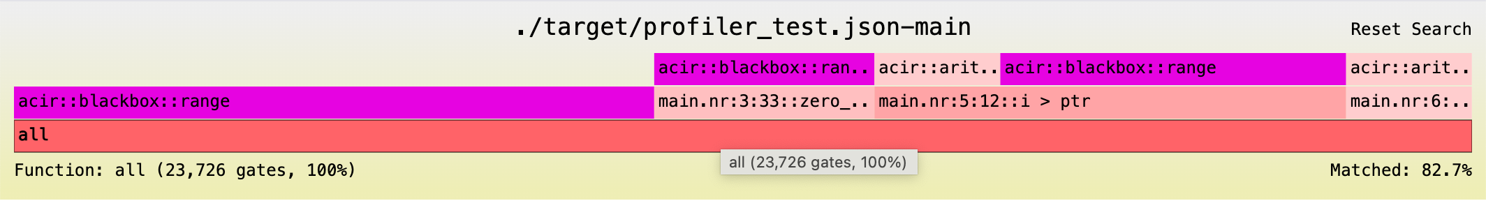
Where blackbox::range contributes a considerably smaller portion of the total proving gates.
Every proving backend interprets ACIR opcodes differently, so it is important to profile proving backend gates to get the full picture of proving performance.
As additional reference, this is the flamegraph of the pre-optimization demonstrative project at array size 32:
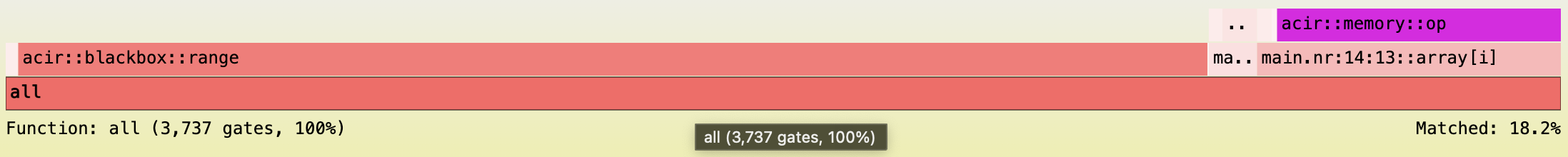
And at array size 2,048:

Profiling execution traces (unconstrained)
The profiler also provides the ability to flamegraph a Noir program's execution trace. This is useful for identifying execution bottlenecks of Noir programs.
The profiler supports profiling fully unconstrained Noir programs at this moment.
Updating the demonstrative project
Let's turn our demonstrative program into an unconstrained program by adding an unconstrained modifier to the main function:
unconstrained fn main(...){...}
Since we are profiling the execution trace, we will also need to provide a set of inputs to execute the program with.
Run nargo check to generate a Prover.toml file, which you can fill it in with:
ptr = 1
array = [1, 1, 1, 1, 1, 1, 1, 1, 1, 1, 1, 1, 1, 1, 1, 1, 1, 1, 1, 1, 1, 1, 1, 1, 1, 1, 1, 1, 1, 1, 1, 1]
Flamegraphing
Let's take a granular look at our program's unconstrained execution trace footprint using the profiler, running:
noir-profiler execution-opcodes --artifact-path ./target/program.json --prover-toml-path Prover.toml --output ./target
This is similar to the opcodes command, except it additionally takes in the Prover.toml file to profile execution with a specific set of inputs.
Flamegraph of the demonstrative project generated with Nargo v1.0.0-beta.2:
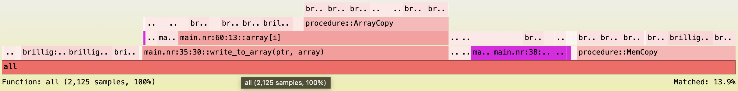
Note that unconstrained Noir functions compile down to Brillig opcodes, which is what the counts in this flamegraph stand for, rather than constrained ACIR opcodes like in the previous section.
Balancing proving and execution optimizations
Rewriting constrained operations with unconstrained operations like what we did in the optimization section helps remove ACIR opcodes (hence shorter proving times), but would introduce more Brillig opcodes (hence longer execution times).
For example, we can find a 13.9% match new_array in the flamegraph above.
In contrast, if we profile the pre-optimization demonstrative project:
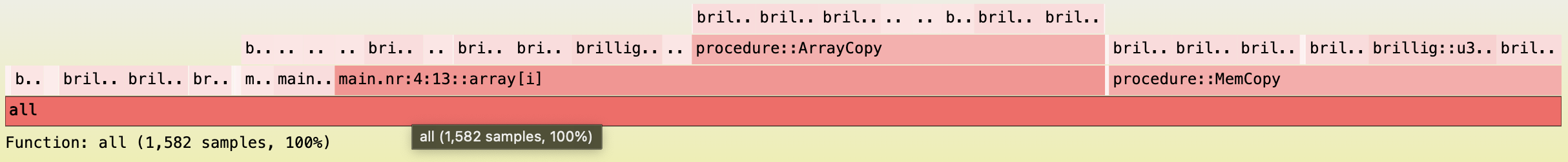
You will notice that it does not contain new_array and executes a smaller total of 1,582 Brillig opcodes (versus 2,125 Brillig opcodes post-optimization).
As new unconstrained functions were added, it is reasonable that the program would consist of more Brillig opcodes. That said, the tradeoff is often easily justifiable by the fact that proving speeds are more commonly the major bottleneck of Noir programs versus execution speeds.
This is however good to keep in mind in case you start noticing execution speeds being the bottleneck of your program, or if you are simply looking to optimize your program's execution speeds.